Comparing STARK provers: Miden and Starknet

Introduction

STARKs (scalable transparent arguments of knowledge) have gained widespread attention due to their ability to help scale Ethereum. They allow one party, the prover, to show to a verifier that a given program execution is correct by submitting proof that can be verified much faster than naïve re-execution by the verifier. The proof size is also smaller, of order $\mathcal{O} (\log^2 (n))$, where $n$ is the number of steps in the computation. Starknet and Polygon Miden use STARKs in their protocols to generate these proofs, using their customized versions. Starknet uses the Stone Prover, while Miden uses Winterfell. Our prover, STARK Platinum in lambdaworks, is a general prover that we want to use as a drop-in replacement for any of these provers. If you want to understand how STARKs work, you can see our previous posts on STARKs, the Stone prover and FRI.

General steps

In a nutshell, STARKs represent a computation using an execution trace (a large table containing the values of the registers during the computation), and an algebraic intermediate representation (AIR), which is a set of polynomial constraints that should be enforced over the trace. STARKs have been improved by leveraging a preprocessing stage and getting randomness from the verifier, turning the AIR into a randomized AIR with preprocessing. This way, we can extend the trace with additional variables that will be useful for memory checks or communicating with a coprocessor. The main steps are:

1. Interpolate the trace columns to get the trace polynomials.
2. Commit to the trace polynomials by evaluating over a larger domain (low-degree extension) and using these evaluations as leaves in a Merkle tree.
3. Optional: sample randomness from the verifier and extend the trace to the auxiliary trace. Interpolate the auxiliary trace columns and commit to these polynomials following the strategy in step 2.
4. Sample randomness from the verifier and compute the composition polynomial using the AIR constraints and the whole trace. Commit to the composition polynomial.
5. Get out-of-domain point $z$ from the verifier, evaluate the trace polynomials and composition polynomial at $z$, and send them to the verifier.
6. Build the DEEP composition polynomial, which will let us check that the evaluations of the polynomials in point 5 are correct.
7. Apply the FRI protocol to the DEEP composition polynomial and get the proof.

Checking constraints

The way we check that the constraints are enforced is as follows: let's denote the rows of the trace as $x_0, x_1, ... x_N$. An element of the trace is simply $x_{ij}$, which is a field element. An AIR constraint is some multivariate polynomial $P(u, v, w)$ where $u$, $v$, and $w$ can be elements from different rows or columns. Each of these constraints also has a validity range. Here there are some examples of constraints:

• Simple boundary constraints: these enforce that a given position in the trace $x_{ij}$ has a prescribed value. For example, we want register $2$ in row $0$ to be equal to 5. The constraint polynomial will be $P (x) = x_2 - 5$. If the trace is valid, when we plug $x_0$ into $P$, we will have $x_{02} - 5 = 0$. If we use some other row, then the polynomial would not necessarily evaluate to $0$.
• Consistency constraints: these enforce that the values of some register satisfy a given condition. For example, if we want register $4$ to be a boolean variable, we need that $x_{k4} (1 - x_{k4} ) = 0$ for all $k$. The constraint polynomial is therefore $P (x) = x_{4} (1 - x_4 )$ and this should hold for all rows.
• Simple transition constraints: show that the value for a register in a row is compatible with the values in the previous row, as dictated by the computation. For example, if we have a sequence $x_{0, n + 1} = x_{0,n}^2 + x_{1 n}$, the constraint polynomial is $P(x_{k + 1}, x_k ) = x_{0,k + 1} - x_{0,k}^2 - x_{1,k}$. The constraints hold for all the computation, except in the last row.
• More complex constraints: these can involve more rows, or be applied only at specific points, which makes their description a bit more complicated.

To enforce the constraints, we need to compose the trace polynomials (obtained by interpreting the trace as evaluations of polynomials over some set $D$) with the constraint polynomials, obtaining as many $C_i (x)$ as constraints we have, and dividing each $C_i (x)$ by their corresponding zerofier, $Z_i (x)$, which is a polynomial that is $0$ where the constraint is enforced. Some zerofiers are:

• Simple boundary constraint: $Z(x) = x - g^k$, where $g$ spans the domain $D$ ($D = { g^0, g , g^2 ... g^{n - 1}} )$.
• Consistency constraints: $Z(x) = x^n - 1$.
• Simple transition constraint: $Z(x) = (x^n - 1)/(x - g^{n - 1})$

The efficiency of the STARK prover depends partly on being able to compute these zerofiers in a fast way. If a constraint were to apply in steps $1, 3, 4, 6, 7, 9, 12, 14, ... n-1$ with no clear pattern, we would have to spend almost linear time trying to evaluate the polynomial. If one wanted to have the simplest prover, it would be best to work with constraints involving at most two consecutive rows and being either boundary, consistency, or simple transition constraints. This helps us reduce the number of zerofiers we need to calculate and the number of multiplications.

The AIR we use and how we organize the trace is important in terms of performance and usability. High-degree constraints in the AIR are going to make the evaluation of the composition polynomial more expensive. On the other hand, having a rigid organization of the trace (trace layout) adds overhead to the proving of general programs and makes it difficult to make changes to the prover. Miden has been developing AIRScript, which is designed to make AIR description and evaluation simple and performant. In Lambdaworks, we are also working to make the definition of AIRs and the evaluation of constraints simpler, leading to faster provers and easier maintenance or updates.

Different Algebraic Intermediate Representations

The AIR for the Miden vm is contained here. The Stone prover's AIR is dependent on the type of layout; the generalities of the AIR are here. This is a list of the different layouts in Starknet:

• Plain
• Small
• Dex
• Recursive
• Starknet
• StarknetWithKeccak
• RecursiveLargeOutput
• AllCairo
• AllSolidity
• Dynamic

Here we show the diagram of a single step of the main trace for the plain layout in Starknet, without the auxiliary trace (for more information, see our analysis):

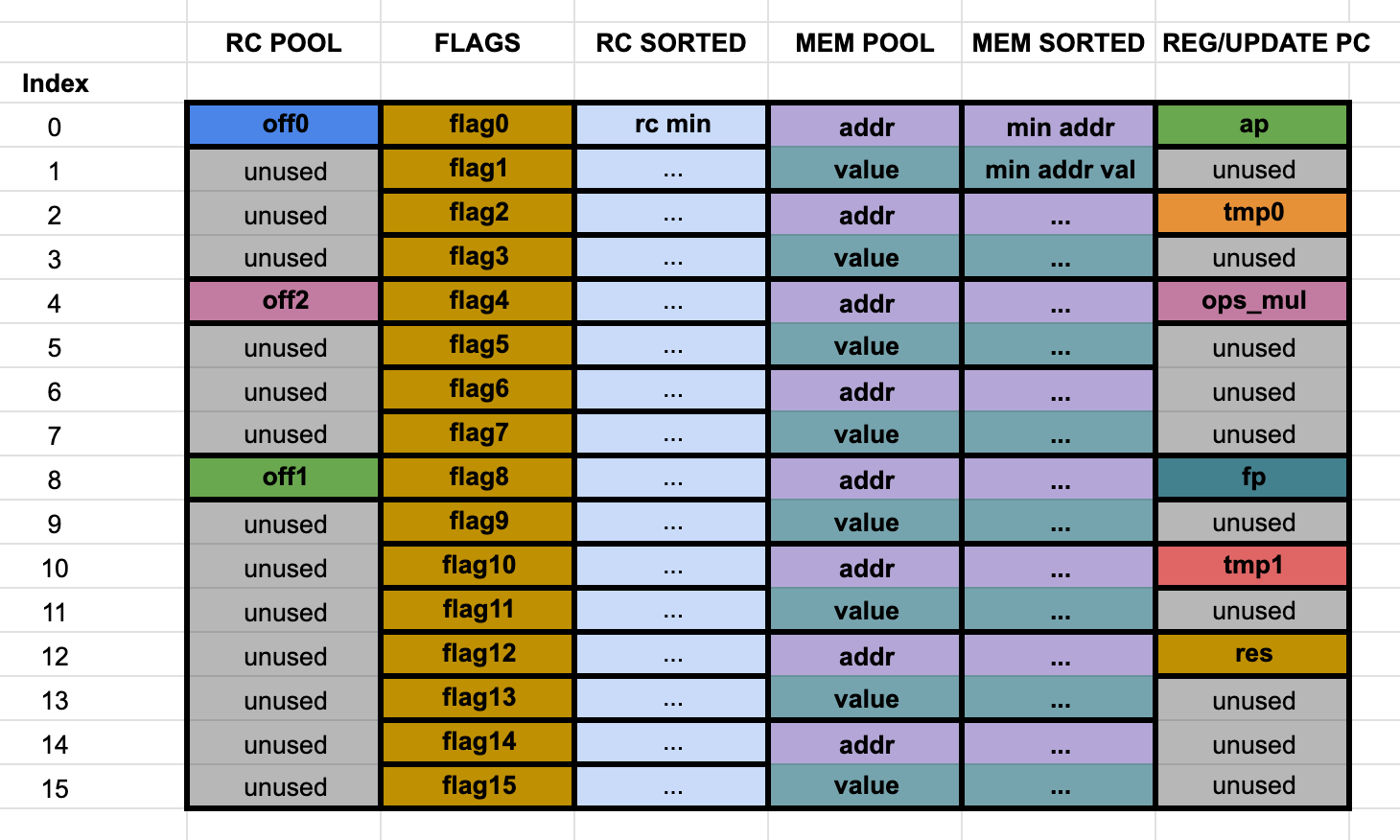
The Stone Prover packs several registers in a single column, creating virtual columns. For example, all 16 flags are grouped under one column. The memory's addresses and values are also grouped in an interleaved way in another column. This reduces the amount of columns in the trace (we merge $16$ columns in $1$), but the trace length becomes $16$ times larger. When we want to find the trace polynomials, we perform one Fast Fourier Transform (FFT) of size $16n$, instead of $16$ FFT of size $n$.

Using virtual columns can be useful if some of the registers are updated only a few times, since we will still have to pad them to full length, reducing memory use in the trace. However, this comes with a big disadvantage: we have to keep different zerofiers and the evaluation frames (which we use to compute constraints efficiently) become more complex. Let's see the difference between both approaches:

16 columns

To evaluate each of the constraints, we need to take just the elements of one row. The trace has length $n$, so the zerofier is $Z (x) = x^n - 1$. 15 flags have the constraint $x (1 - x) = 0$, while the last one has $x = 0$.

Single virtual column

To evaluate each constraint, we need to take just one element from the row. The problem is that the constraint $x (1 - x)$ is valid for all rows, except every $16$-th row, while constraint $x = 0$ is valid only for every $16$ rows. This way, we have to maintain two zerofiers, one for each constraint:

• $Z (x) = (x^{16n} - 1) / (x^n - g^{15n/16})$
• $Z (x) = x^n - g^{15n/16}$

The other problem is that, if a constraint involves several flags, we need to pass several rows to be able to evaluate it. It is worth noting that $g$ in this case is different from the previous case, as the interpolation now takes place over a domain of size $16n$.

Built-ins and chiplets

Having a general-purpose CPU for proving comes with a cost: the virtual machine is not optimized for some commonly used operations. To deal with this, the Cairo vm (Starknet) and Miden vm introduce coprocessors to deal with these operations and then communicate the results to the CPU.

Chiplets and the Miden vm

Miden uses dedicated components to accelerate complex computations, called chiplets. Each chiplet handles a unique computation and is responsible for proving the correctness of the computation and its internal consistency. Currently supported chiplets are:

• Hash
• Bitwise
• Memory
• Kernel ROM
• Range checker (it works as a chiplet, but it is handled separately)

The chiplets execution trace is built by stacking the execution traces of each of the chiplets. This is an optimization since each chiplet is likely to generate fewer cells than other components of the vm, avoiding significant padding to take them to the same length and reducing the number of columns. It uses a similar reasoning to virtual columns in Stone, but it does not interleave them.

Chiplets are identified by selectors. The total degree of the constraints is between $5$ and $9$ and each chiplet takes between 6 and 17 columns. The selectors are:

• $1$: hash
• $1,0$: bitwise
• $1,1,0$: Memory
• $1,1,1,0$: Kernel ROM
• $1,1,1,1$: padding

Stacking the traces of the chiplets has some difficulties, though, since the consistency and transition constraints in the last row of one chiplet may conflict with the first row of the next chiplet. This is the case of the memory and kernel ROM chiplets, where selector flags solve the conflicts.

The chiplets are connected to the rest of the VM using a bus, which can send requests to any of the chiplets and receive a response. It is implemented as a running product column and, if the requests and responses match, the bus will begin and end with $1$.

One of the main drawbacks of this approach is that the constraints have a rather large degree, which makes constraint evaluation more expensive. On the other hand, the construction does not require handling several zerofiers and looks simpler to implement and understand.

Built-ins and Cairo vm

Built-ins are application-specific AIRs that can reduce the size of the execution trace of a given computation. For example, expressing the Poseidon hash function using Cairo needs 35k cells in the trace, while the Poseidon built-in reduces this to roughly 600-650 cells. Among the built-ins, we have:

• Poseidon
• Pedersen
• Elliptic curve operation
• Keccak
• Bitwise
• ECDSA
• Range check

The integration of the built-ins needs some care, though, as naïve ways may result in wasting cells, reducing the efficiency of the construction. Layouts specify the amount of cells and positions that are allocated to each component. Depending on the type of program we want to prove, we can select from the different layouts offered in Starknet to achieve the most cost-effective solution. However, it may be the case that the existing layouts provide significant overhead to prove our program, as noted in the discussion of dynamic layouts. Adding new layouts needs expert knowledge and careful analysis; it may also be confusing to users, who need to understand the differences between the layouts.

Each built-in has a memory segment. To check that there is no overflow from the memory segment, there are two pointers (start and stop) that are exported via the public memory mechanism. Since the constraints for each built-in apply every several rows, we are forced to compute different zerofiers and handle more complex evaluation frames.

Conclusion

In this post, we discussed the characteristics of STARK provers and some implementation trade-offs. We analyzed how the Miden and Cairo VMs handle their execution traces and the description of the AIR. We also discussed the main types of constraints and the way to enforce them over the execution trace. The use of virtual columns (grouping several registers in one column) reduces the number of FFTs we have to perform, but it comes at the expense of more complex evaluation frames and keeping several zerofiers. However, this strategy is necessary when several components have fewer trace cells and padding is necessary. Miden uses this type of strategy when dealing with chiplets, but it chooses to stack the traces instead of interleaving them. This introduces several selector variables, which increase the degree of the constraints, adding an extra cost to constraint evaluation. On the other hand, evaluation frames are simpler and we do not have to compute several zerofiers. The use of layouts could lead to a more cost-effective solution, though at the expense of a larger overhead to prove some types of programs. Besides, adding more layouts increases complexity and makes things harder to maintain. We like analyzing the different solutions and their trade-offs, as they could lead to new designs that can help us improve general-purpose provers.