Proof aggregation techniques
Proof aggregation techniques
Introduction
SNARKs (succinct, non-interactive arguments of knowledge) and STARKs (scalable, transparent arguments of knowledge) have gained widespread attention due to their applications in decentralized private computation and scaling blockchains. They are tools that allow us to prove to another party that we did a computation correctly so that the verification is much faster than re-executing the computation. The size of the proof is much smaller than all the information needed to prove it. For example, we can prove that we know the solution to a Sudoku game without fully providing it. In the case of the execution of a virtual machine, to prove correctness, we should see how the machine's registers change at every cycle; the verifier does not need to know it completely but rather queries the registers at some point. For a discussion on the impact of SNARKs/STARKs, see our post.
Proving large programs or computations can be expensive since this introduces an overhead in running them. In some cases, the computation can be broken down into several smaller computations (for example, proving the transactions inside a block can be done by proving each transaction separately), but this has two drawbacks: proof size and verification time scale linearly with the number of components. Both hurt scalability because we need more time to verify the entire computation, and it increases memory use. We can solve this by bundling all the proofs and doing just one verification. We can use several techniques; the best one will depend on the type of proof system we use and our particular needs. This post will discuss some of the alternatives we have and their tradeoffs in terms of prover time, verification time, and proof size.
Aggregation techniques
These techniques will allow us to prove several statements together, reducing the blowup in proof size and verification time introduced by checking several statements. For an explanation of some techniques, see the following video.
Proof recursion
SNARKs/STARKs let us check the validity of any NP statement in a time- and memory-efficient way. The amount of information needed to prove a statement is much smaller than the size of the required witness to check the statement. For example, in STARKs, the verifier does not need to see the whole execution trace of the program; it just needs some random queries. In Plonk, the verifier has the evaluations of the trace polynomials at a random point, which is much less than the $3n$ values in the trace.
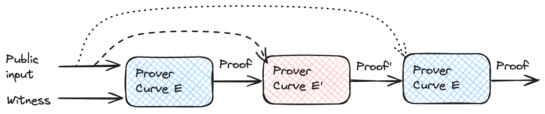
How does recursion work? The prover proves that he verified a proof $\pi$ corresponding to some computation with public input $u$. The image below shows the flow for recursion.
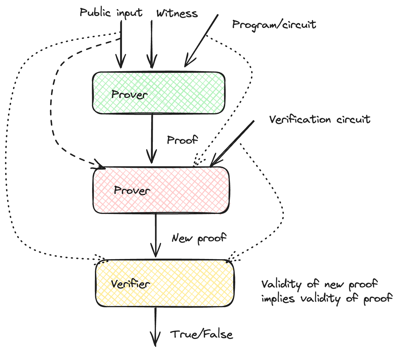
The prover takes the public input, the witness, and the program and generates the proof $\pi$ attesting to the validity of the computation. The prover then takes the proof $\pi$ and original circuit as witnesses, the public input, and the verification circuit (the operations the verifier would have to do to check the statement) and obtains a new proof $\pi^\prime$, showing that the prover knows the proof $\pi$ which fulfills the verification circuit with the given input. The verifier can check the proof $\pi^\prime$, which shows that the verification done by the prover is valid, which in turn implies the correctness of the first computation. In the case of STARKs, if the trace for the verification operation is shorter than the trace for the original program, proof size and verification time are reduced (since they depend on the trace length, $n$).
We can also use two different provers. For example, we can prove the first program with STARKs, which is fast but has larger proofs, and then use Groth 16/Plonk, which has smaller proof sizes. The advantage is that the second case does not need to handle arbitrary computations, so we can have just one optimized circuit for STARK verification. The result is one small proof with fast verification.
We can also use the same structure and prove the verification of several proofs.
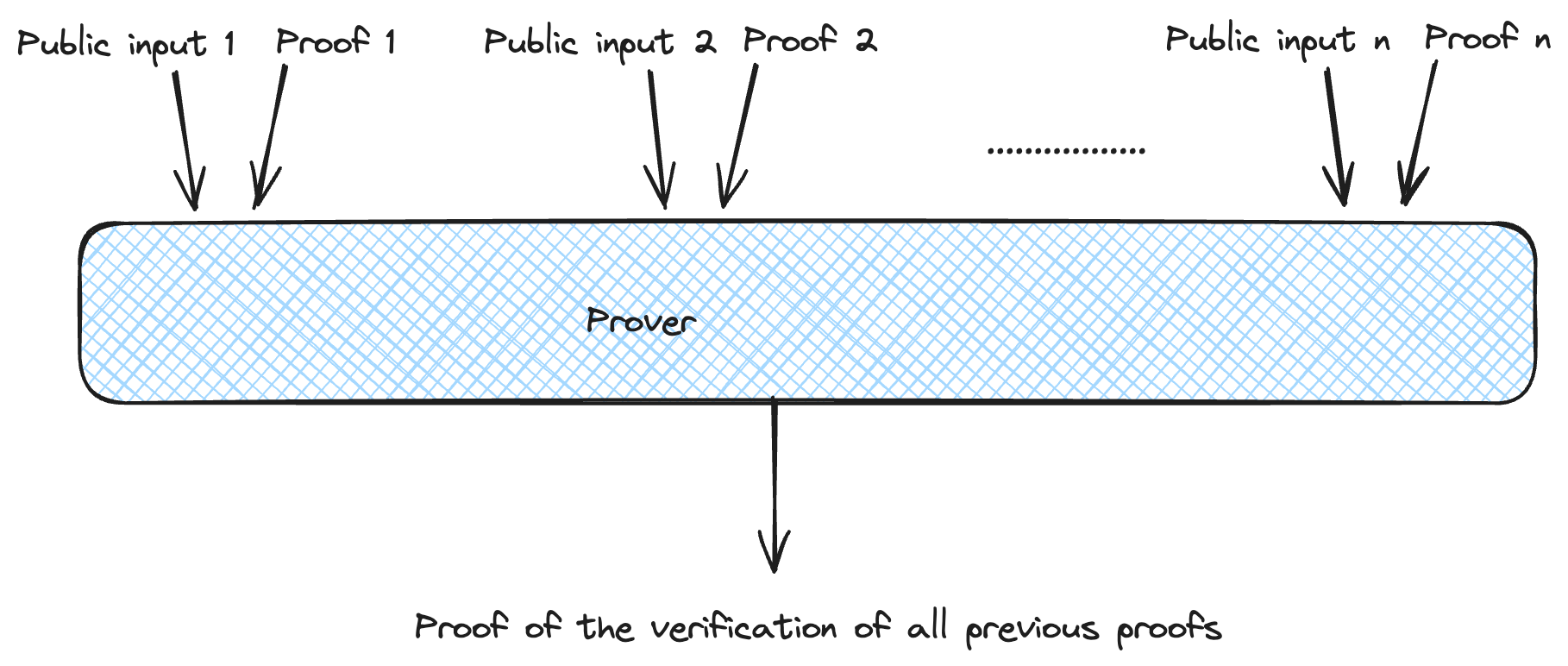
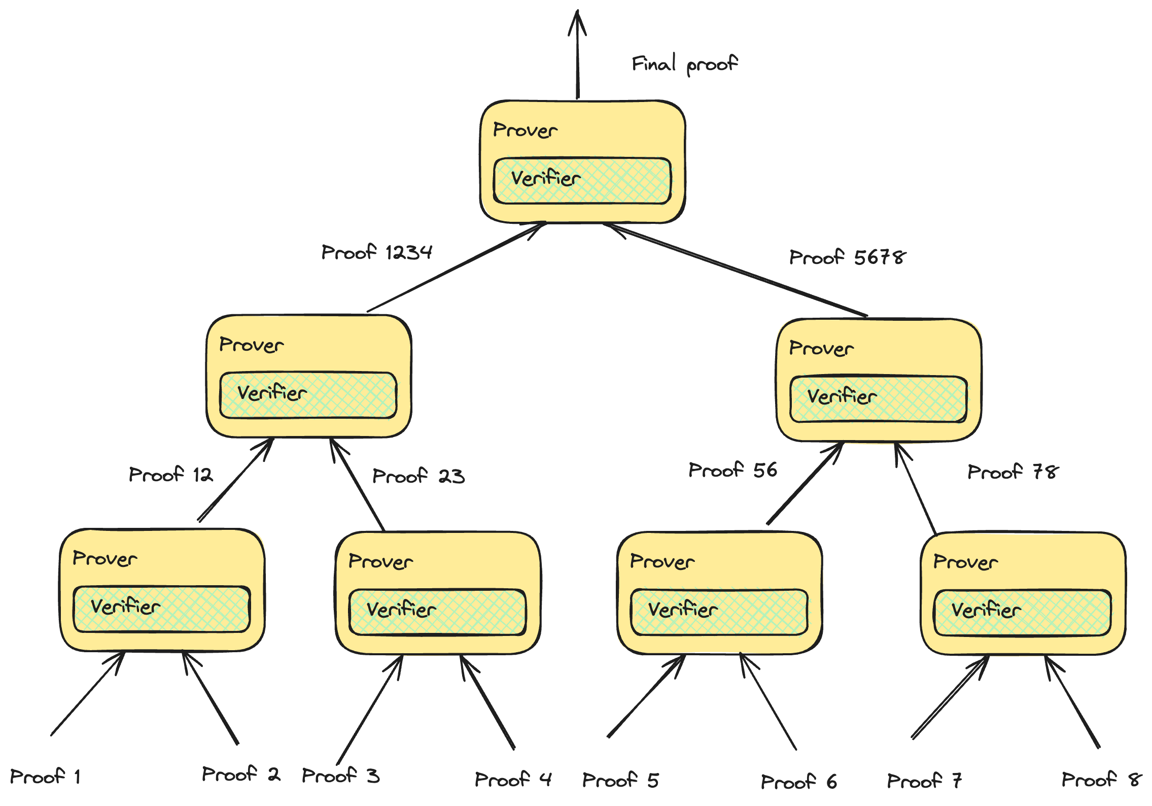
One problem we face is that even though the proof size is reduced, the public input increases linearly. We can solve this by providing a hash/commitment to all the public input and passing it as part of the witness. During the verification, we have to check that the hash of the public input in the witness corresponds to the hash/commitment of the public input. Proof recursion can be handled more efficiently by building a tree structure, increasing the degree of parallelization.
Proof recursion is used in several projects to reduce proof size and make verification cheaper, such as Starknet, Polygon ZKEVM, and zkSync.
Even though proof recursion has many advantages, it adds workload to the prover. In proof systems such as STARKs, the prover has to compute lots of hashes, which are expensive operations. Luckily, there have been advances in algebraic hash functions (less costly to prove) and protocols such as STIR that reduce the number of hashes needed to generate proofs (post coming soon). In SNARKs working over elliptic curves, the proofs consist of elements in the curve (with coordinates over a field $F_p$) and scalar represented in $F_q$ (the scalar field). This generates a problem since we have to do operations over $F_p$ to compute operations over the curve. Still, the scalars in the circuit live in $F_r$, leading to non-native field operations. Here you can find a circuit to verify Groth 16 proofs, taking around 20 million constraints. As discussed in the following section, curve cycles are a nicer alternative to avoid field emulation.
Cycles of curves
We have the problem that coordinates for the curve $E$ live in $F_p$, but the scalar field is $F_r$. If we can find a curve $E^\prime$ defined over $F_r$ and scalar field $F_p$, then we could check proofs over $E$ using $E^\prime$. Pairs of curves with these characteristics are called a cycle of curves. Fortunately, some curves of the form $y^2 = x^3 + b$ satisfy the conditions. Pallas and Vesta curves (known together as Pasta curves) form a cycle and are used in Mina's Pickles and Halo 2. We covered some of the basics of Pickles in our previous post. Pickles uses two accumulators (each using a different curve) and defers some checks to the next step. This way, it can avoid expensive verifications and efficiently deliver incrementally verifiable computation.
Folding and accumulation schemes
One of the drawbacks of full recursion is that we need to prove the whole verification, which can be very expensive. For example, in recursive STARKs, we must compute all the hashes and verify all algebraic operations to get to a new proof. Folding schemes provide an alternative to full verification by combining several instances and accumulating them. Nova introduced a folding scheme for R1CS. The key idea is that if we have two solutions $(u_1 , w_1 )$ and $(u_2 , w_2 )$ for R1CS, we can combine them into a single claim $(u , w)$ for a committed relaxed-R1CS (a generalization of R1CS).
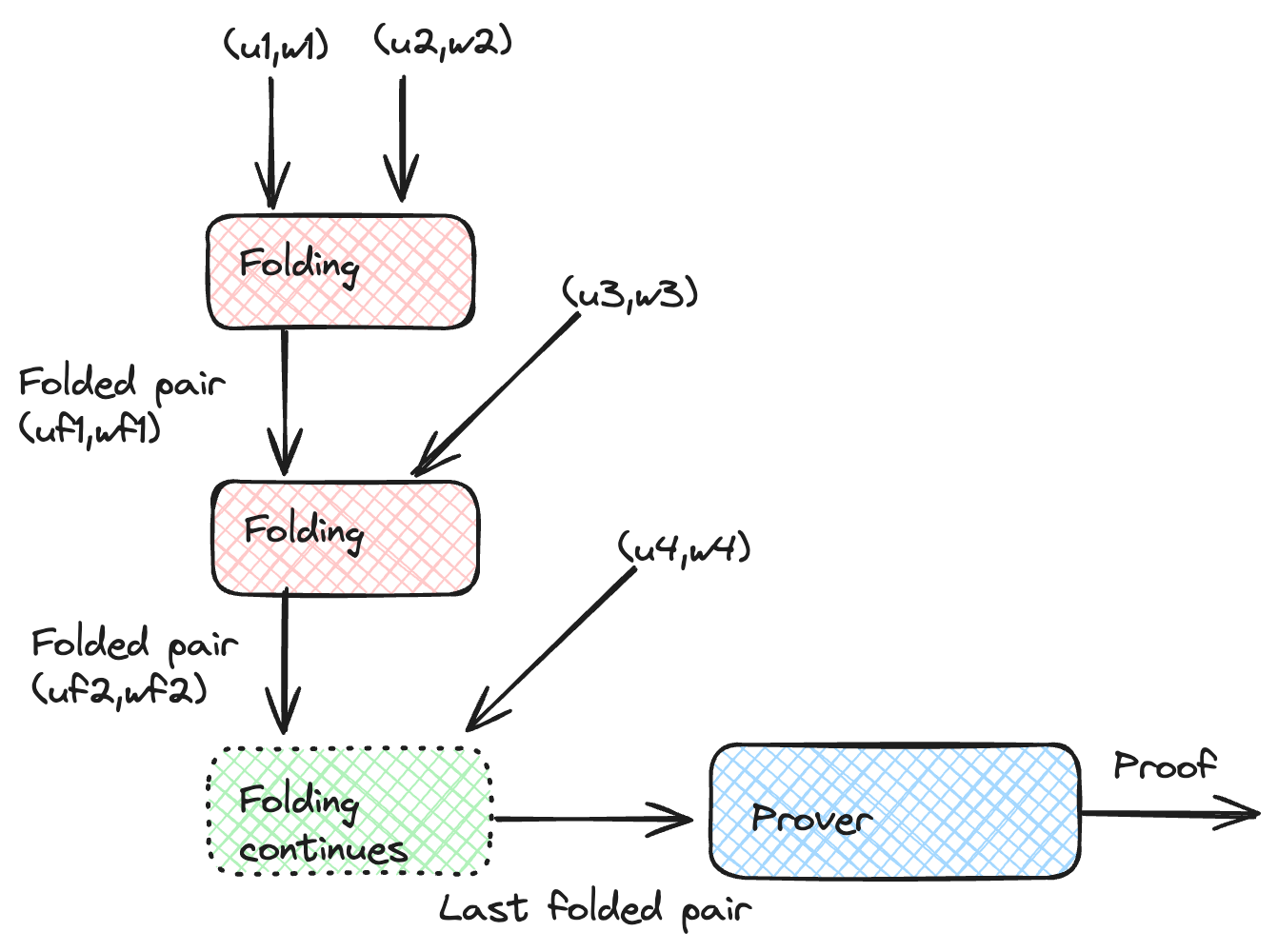
We can then generate a proof for the unified claim, which amounts to the validity of all instances.
SNARKPack
Some proof systems have proofs that can be aggregated by other methods, such as SNARKPack for Groth 16. The proof for Groth 16 consists of three elements $\Pi = (\pi_1 , \pi_2 , \pi_3)$, where $\pi_1, \pi_3$ belong to the group $G_1$ of an elliptic curve and $\pi_2$ belongs to $G_2$. The check in Groth 16 is the following pairing equation,
$e(\pi_{1} , \pi_{2} ) = Y e(\pi_3 , D)$
where $Y$ depends on the public input and the parameters of the ceremony, and $D$ is part of the parameters. If we have several proofs $\Pi_k = (\pi_{1k} ,\pi_{2k}, \pi_{3k} )$, we can combine the different checks,
$e(\pi_{1k} , \pi_{2k} ) = Y_k e(\pi_{3k} , D)$
using random numbers $r_k$ such that
$\prod e(\pi_{1k} , \pi_{2k} )^{ r_k } = \prod Y_k^{ r_k } \prod e(\pi_{3k} , D)^{ r_k }$
We can rewrite this as
$Z_{AB} = Y^\prime e(Z_C , D)$
where
$Z_{AB} = \prod e(\pi_{1k} , \pi_{2k} )^{ r_k }$
$Y^\prime = \prod Y_k^{ r_k }$
$Z_C = \prod \pi_{3k}^{ r_k }$
The verifier needs to check that $Z_{AB}$ and $Z_C$ are consistent with the proof triples $\Pi_k$ provided. This is done via a target inner pairing product and a multiexponentiation inner product. The advantage is that the combined proof size is practically independent of the number of proofs aggregated.
Continuations
Continuations are a mechanism by which we can split a complex computation into smaller segments that can be computed and proven separately. This enables faster proving by leveraging parallelization and reducing the provers' memory footprint. The downside is a blowup in proof size unless implemented in rollup form. However, let's take advantage of the independent proofs and use a folding scheme to combine all the claims to the same verification circuit or recursive proving. We can wrap all the segments into a single proof (which could also be a SNARK with constant proof size).
Summary
Over the last decade, we have seen the development of new proof systems and techniques to show the validity of computations in a memory- and time-efficient way. However, we need to break down large computations into smaller, independent computations (for example, proving a block of transactions by proving each transaction separately). The downside is that we have a blowup in proof size and verification time, which can hurt scalability or increase costs. Luckily, there are several techniques for aggregating proofs, so verifying a single proof implies the validity of all the other proofs. While proof recursion offers a highly parallelizable way to aggregate proofs, it involves costly operations, such as field emulation and hash functions. Accumulation or folding schemes provide an alternative to full verification by deferring some checks until a final verification step.
