Scientific Machine Learning with Julia: the SciML ecosystem

Interview with Chris Rackauckas

We live in a complex world. For those scientists who dare to immerse themselves in that complexity and generate a deeper understanding of it, it is very common to have to deal with differential equation models that are not possible to solve without the use of a computer.

A lot of time is usually be spent in coding the particular differential equation for each problem. Julia SciML works to create and maintain tools that improve this process— from the creation of a framework that allows to automate the pipeline to create and solve problem-specific differential equations with a high level syntax, to introducing machine learning methods to infer unknown components of the model, and many other functionalities.

We interviewed the creator of SciML, Chris Rackauckas, to get to know a little more about his work.

Please tell us a bit about yourself. What is your background? what is your current position?

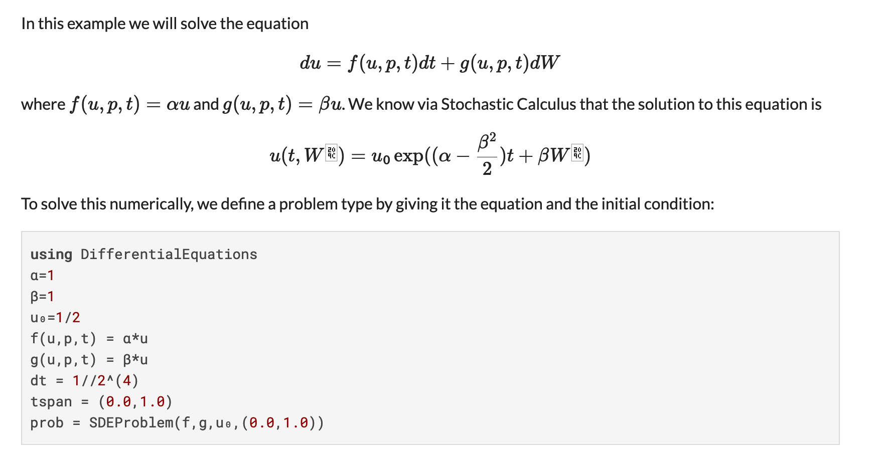
I am an applied mathematics instructor at MIT, the Director of Scientific Research at Pumas-AI, and a senior research analyst at the University of Maryland, School of Pharmacy. My background is numerical differential equations and systems biology, where my PhD was in new methods for efficient solving of stochastic differential equations to model the control of randomness in the developing zebrafish hindbrain.

What is SciML? Why was it born and what’s its purpose?

Before the “SciML” organization, there was just DifferentialEquations.jl and JuliaDiffEq, but it grew beyond just a single project. There were methods for symbolically manipulating equations, sparse automatic differentiation, automated model discovery, neural PDE solvers, and even packages in Python and R for using these tools. So the name didn’t fit and we did a reorganization around the central principle: scientific machine learning. Scientific machine learning is a burgeoning field that mixes scientific computing, like differential equation modeling, with machine learning. That is the essence of the organization: many tools for scientific simulation with differential equation solvers, chemical reaction network tools and N-body simulators, but all of them can compose with machine learning.

Scientific Computing and Machine Learning are often perceived as very different areas. What would you say are the strengths and weaknesses of each one and how does SciML take advantage of them?

Scientific computing generally requires a lot of prior knowledge about the system. You need to be able to create a “mechanistic model”, which requires knowing the physical laws, the chemicals which react, or other way to mathematically encode each interaction of the system. If you know this, great! Then you have a very predictive model. You might know all of the chemicals which interact but not know the reaction rates, and then 12 data points can turn this into quite a predictive model. So these models are interpretable (since it’s all about the mechanism), data efficient, etc. They are great at extrapolating too: the theory of gravity gives pretty good predictions for what happens on Earth as it does for the solar system as it does for galaxies.

Data-driven modeling, like machine learning, takes a completely opposite approach of being “data first”. You have a non-mechanistic model, and you “train” the model based on the data. This requires a lot of data, but you can do this even when you have no idea what the mechanism is. What’s the mechanism for what movie someone will want to watch next on Netflix given the previous movies they’ve seen? Einstein didn’t have a theory for that! But with big data, you can generate such a model.

Scientific machine learning is about pairing together these two paradigms. Incorporating mechanism into machine learning makes it more interpretable, more data efficient, and better able to predict beyond the training data, all without requiring that you know all of the mechanisms. We’re using this in cases like pharmacometrics, where in the first clinical trial we may not know everything about how the drug works, but we can start with a pretty good guess by using mechanistic models derived for similar drugs, and use the incoming data to train models which transforms the prior model towards the data.

What are Neural ODEs? When is it appropiate to work with one? Do you fear that accuracy or interpretability is lost by introducing a Neural Network as part of the equation? Aren’t there other learning methodologies suited for such a thing?

Neural Ordinary Differential Equations or Neural ODEs are ordinary differential equations defined by a neural network. Indeed the result is less interpretable than having a mechanistic physical model, but it allows for the model to be learned directly from data. The neural network makes it not just estimating parameters, but estimating functions. As a middle ground, we created the universal differential equation which is a partially mechanistic model where the neural networks fill in areas of the model which are unknown or have a lot of uncertainty. In this sense, there is more of a continuum between the data-driven and mechanistic models.

Currently, there exist many differential equations solvers, why do you think this is the case? Is there a way to choose the best one for each situation?

We created an automated algorithm chooser in order to mitigate this issue. If you do 'solve(prob)' (i.e. don’t specify a solver algorithm), it will choose one for you. Then you can give it hints to go down different branches. As time goes on I think we will keep refining that algorithm and pushing more people towards that.

What are the key reasons the SciML Differential Equations solver is so fast? How does it differ from others? How influential was writing it in Julia?

Every differential equation solver specializes on some aspect of the differential equation, giving them different performance aspects. For example, BDF integrators, “the standard” for stiff equations, use values from past steps. This can speed things up if the equation is not too stiff, but if it’s too stiff then you cannot use a high order (known as the Dahlquist barrier) and it slows down. So it’s problem dependent as to how well it can mitigate numerical issues, which means for some problems it’s fast and in others it breaks down. Then, if you have discontinuities which are frequent, like dosing in pharmacometrics simulations, this also requires order reduction and thus makes this particular method slower. DifferentialEquations.jl has about 300 methods when you consider all of the tableaus across not just ODEs but also SDEs, DAEs, and DDEs, and it’s this collection that allows it to be efficient.

Regarding the importance of being able to quantify the uncertainty of the numerical resolution when solving differential equations, how does SciML address this problem?

DifferentialEquations.jl comes with a module DiffEqUncertainty.jl that gives sampling-based estimates of numerical uncertainty by causing jitter on the order of the error estimates calculated on each step. Normally these error estimates are only used for adapting dt, but this gives a way to get essentially a free estimate of what other possible paths look like. Andrew Stuart’s group at CalTech then has a full publication that describes that this method indeed matches the error distribution of the full solve. So if you run this a hundred times you’ll get a sense of what all of the possible trajectories could’ve been given the error tolerance that you allowed.

What are MultiScaleArrays? In what ways do these data structures help us in simulating complex scientific models?

The differential equation solvers, and actually all of the SciML ecosystem, work on abstract interfaces which allow for the concrete implementation of a type to be radically different from the standard implementation. MultiScaleArrays is a nice example of this where an entire multi-scale model is represented as both a graph structure and an array simultaneously. This lets the user write a model like “for every cell in the lung, do the chemical reactions of a lung cell” to define a model, but have the stiff high-performance ODE solver automatically know how to interact with this object. It’s not even an array: it’s an array of arrays of arrays etc., which acts like an array. In this form it’s very efficient to allows cells to divide and die, and the ODE solver will adapt the size of the solution vector automatically as this changes.

While this was made for the specific case of multi-scale biological modeling in mind, other users have since come up with other great examples. CuArrays are CUDA-accelerated arrays that live on the GPU that can be dropped in as a replacement to the standard array, or ComponentArrays.jl defines an array type similar to MultiScaleArrays which is backed by a real vector, so it’s faster for standard computations but slower for size changes. A lot of new features can thus be directly added and optimized in the ODE solver just by changing the input types!

Are the processes of solving differential equations and training a Neural Networks similar? How do you put together both frameworks?

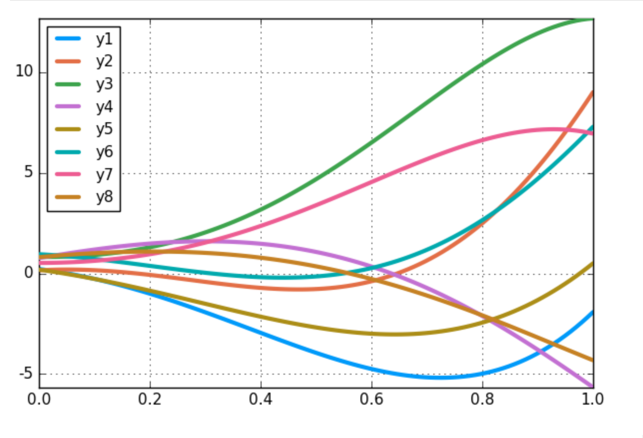
Training a neural network is solving an ODE defined by the gradient of the loss function until zero. Solving that ODE with Euler’s method is gradient descent. So you could use an ODE solver as the algorithm for training a neural ODE, and there is a use case that we’re looking into for that. Differential equations are more ubiquitous than I think most people realize.

Is GPU computing integrated in the SciML ecosystem? How important is having this feature to a scientific computing framework nowadays?

Yes, there’s two major ways. If you have “big kernels”, like PDE solving or neural networks integrated into models, you can do those calculations on the GPU. This is what’s known as “within-method parallelism”. One of the more recent techniques that we have is “between-method parallelism”, where we can automatically generate CUDA kernels from your model and parallelize that between trajectories of the solution. This uses some fancy code generation tricks thanks to tools like KernelAbstractions.jl, and allows “small problems” to have an effective way to use GPUs as well.

How important is it? Somewhat. There are problems which are extremely GPU-parallelizable, like neural ODEs and PDEs, and there are problems which are not, like lots of semi-mechanistic universal differential equation models. Whether a GPU is useful is very dependent on what and how you’re trying to model.

In which cases is it worth to add a Bayesian analysis to the parameter estimation, for example with the use of DiffEqBayes.jl? What are its advantages over more classical optimization algorithms?

Bayesian analysis gives you a posterior distribution which has a sense of uncertainty quantification, i.e. it doesn’t just give you the “best parameter” but also a distribution which you can use to understand the error bars on your parameter estimate. In many cases this is a fundamentally interesting quantity. For example, in pharmacology we often want to know the probability that the drug concentration is in the safe zone. To evaluate this, we need a probabilistic fit of the model since only by including the uncertainty of our parameters can we get an accurate guess of the probabilities of the dynamics.

Are there any relevant books or papers you would like to recommend for digging deeper in these topics?

Books schmooks. You’ll want to go directly to the sources. The only books I really recommend these days are Ernst Hairer’s “Solving Ordinary Differential Equations” I and II tomes: those are a work of art. Also Kloeden’s book on numerical methods for stochastic differential equations. Other than that, dive right into the scientific literature.

What is next for SciML? Are you currently working on some other features to add in the near future?

There’s tons we’re doing! I think a lot of what’s next is the integration of symbolic computing into all of our tools. ModelingToolkit.jl is the centerpiece of that push, and while I gave a talk at JuliaCon 2020 showcasing how it can be used as an automated code optimization tool (and gave a PyData 2020 talk on how you can GPU-accelerate ODE solves in R using it!), it’s so much more than that. It’s sometimes hard to numerically do things correctly, like ensuring positivity in an ODE solution can be difficult. But if you log transformed your model, then by definition your solution will always be positive. Right now this is up to the user, but what if we could automatically change the equations you wrote so that, not only are they more efficient, but they are also mathematically easier to solve and estimate? That’s the scope of ModelingToolkit, and if that interests you then you might want to stay tuned to that and its sister product NeuralSim which is about automated surrogate acceleration for the ModelingToolkit modeling language.